Educational tool; results are estimates for learning, verify with your textbook or instructor.
This page computes probabilities for a normal model with mean $\mu$ and standard deviation $\sigma$. Raw score mode takes those two numbers and a range: below an upper bound, $P(X<b)$, above a lower bound, $P(X>a)$, or between two values, $P(a<X<b)$. Each bound is standardized with $z=(x-\mu)/\sigma$, then read from the standard normal CDF. Standard normal mode approximates $\Phi(z)=P(Z\le z)$ for $Z\sim N(0,1)$. Inverse mode turns a percentile into a cutoff. With mean $0$ and standard deviation $1$ that cutoff is a $z$ score. With any other mean and a positive standard deviation it is the raw score $x=\mu+z\sigma$.
The number is meaningful when a normal model is already justified. Many school tables stop at two decimals of $z$. This page is a smoother table that also accepts the mean and the standard deviation. It evaluates a model you have already chosen.
CDF uses an error function approximation from Abramowitz and Stegun (formula 7.1.26) via $\Phi(z)=\tfrac12(1+\mathrm{erf}(z/\sqrt{2}))$. The inverse uses a rational approximation in the style of Acklam and Beasley Springer. Treat the digits as educational. A statistics package belongs in a high stakes setting.
How to use the three modes
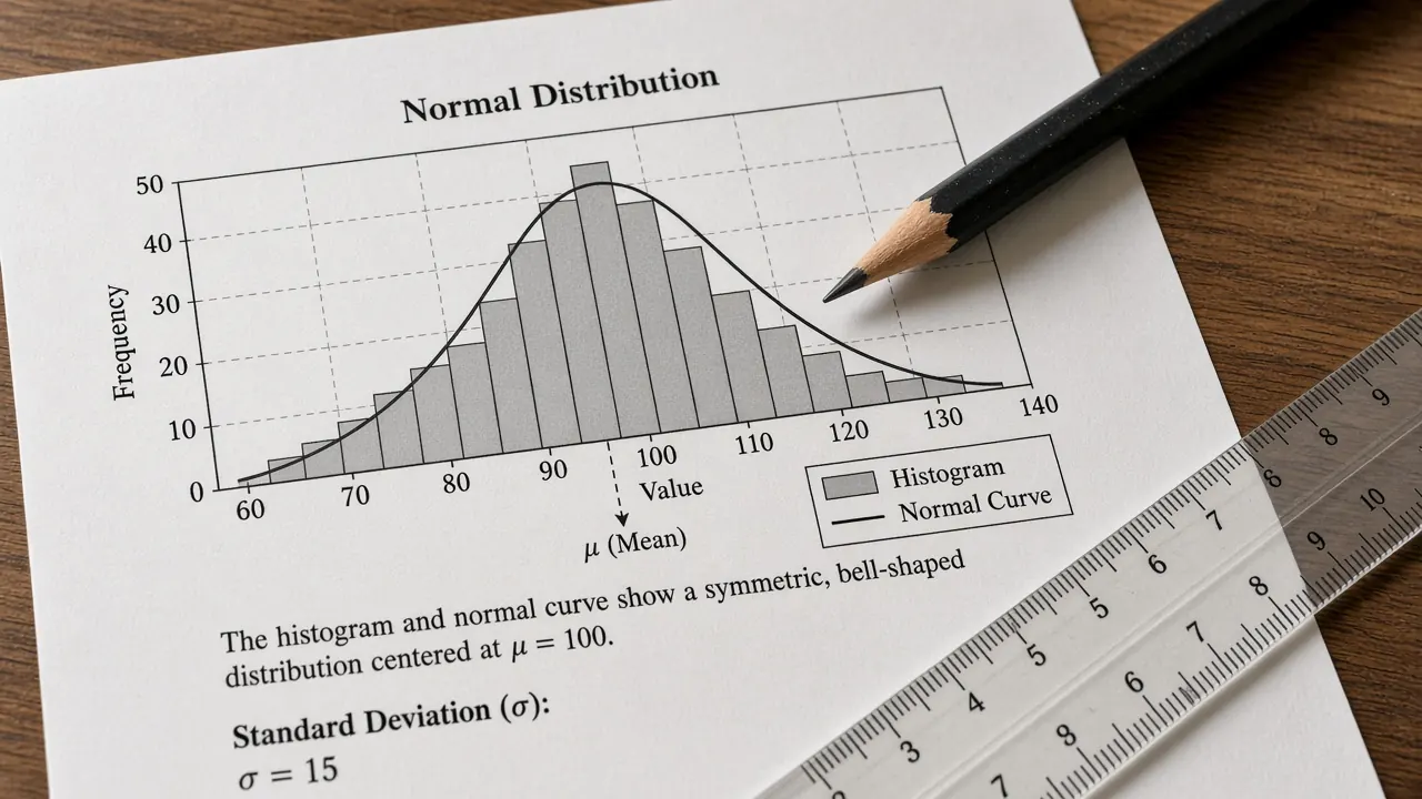
Raw score mode is the default. Enter the mean, a standard deviation greater than 0, and the probability you want: below an upper bound, above a lower bound, or between two bounds. The defaults are mean 100, standard deviation 15, and the probability between 85 and 115. Press Compute, or press Enter from any box. The lines under the answer show $z=(x-\mu)/\sigma$ for each bound, then the probability in words.
Standard normal mode sets the mean and the standard deviation aside. Type a $z$ score. The default $1.96$ should land near $0.975$, the familiar left tail at the edge of a two sided $95\%$ interval.
Inverse mode turns a left tail probability into a cutoff. A number above $1$ is read as a percentage, so $97.5$ and $0.975$ ask for the same place on the curve. Mean $0$ and standard deviation $1$ return a $z$ score. Any other mean, with a positive standard deviation, returns the raw score $x=\mu+z\sigma$. Inverse mode keeps its own mean and standard deviation. Switching modes does not copy the raw score boxes into the inverse boxes.
How to read the output
The large number is the probability, or the cutoff in inverse mode. The lines underneath substitute your inputs into $z=(x-\mu)/\sigma$ and then into $\Phi$. A probability between two values is $\Phi(z_b)-\Phi(z_a)$. A left tail is $\Phi(z)$. A right tail is $1-\Phi(z)$.
A left tail answers how much of the model sits below the bound. A two sided interval uses both tails, and you add those yourself. A right tail of $5\%$ is a left tail of $95\%$.
On a continuous curve, the probability of one exact number is 0. The page prints strict inequalities. The inclusive version, with $\le$ or $\ge$, is the same number.
Two worked examples
The middle band of a placement test
A placement test is modeled as normal with mean 100 and standard deviation 15. The band from 85 to 115 sits one standard deviation on either side of the mean. Leave the page on raw score mode, keep those four numbers, and choose the probability between two values. The standardized ends are
$$z=\frac{85-100}{15}=-1,\qquad z=\frac{115-100}{15}=1.$$
The probability is $\Phi(1)-\Phi(-1)$, about $0.6827$. Roughly 68 percent of this model falls in that band. That is the middle slice of the empirical rule, checked from the curve. Including the scores 85 and 115 themselves does not move the probability, because a continuous model gives one exact score probability 0.
From 1.96 back to a raw cutoff
Switch to standard normal mode and enter $1.96$. The left tail $\Phi(1.96)$ is about $0.9750$, so about 2.5 percent of a standard normal sits above $1.96$. Inverse mode runs that fact backwards. Leave the mean at $0$ and the standard deviation at $1$, and type $97.5$. The cutoff returns near $1.96$.
The same percentile on the placement test uses mean $100$ and standard deviation $15$ in inverse mode. The page returns $x=\mu+z\sigma$, a bit under $129.4$. About 97.5 percent of that test model sits at or below that score.
Common pitfalls
The standard deviation has to be greater than 0. A blank box, a zero, or a negative value stops the page with a message. For a probability between two values, the lower bound has to sit below the upper bound. Equal bounds are allowed, and the probability is 0.
Percentiles and $z$ scores are different boxes. Typing $97.5$ in standard normal mode treats it as a $z$ score, far in the tail. Typing it in inverse mode treats it as a percentage. Typing $0.975$ and typing $97.5$ in inverse mode are meant to agree.
Accuracy is weaker far in the tails than near the mean. The documented error of the erf approximation is small, and it is still an approximation. Use a statistics package when a decision is high stakes.
A normal curve is a model. Data that are skewed, discrete, or bounded can make these probabilities a poor summary even when the arithmetic is fine.
Related reading
Place the model on probability and statistics. Nearby language: random variable, expected value, and probability. Belief updates after evidence are on the Bayes theorem calculator and in Bayes theorem without the fog.
A discrete two outcome model is the binomial probability calculator. Counting is on the combinatorics calculator.